| <–AI-potential and drawbacks | Speaking humans and machines–> |
Machine Learming is an area of AI which has emerged as a leading tool for data analysis because of its ability to learn directly from raw data, with minimal human intervention [2]. The main scope of a ML application is to automatically detect meaningful patterns in data, to make subsequent predictions about new data [3]. ML comprehends several strategies to reach this goal, which are called learning models. In this chapter, after a short introduction on how the brain works, we will introduce recent Deep Learning (DL) approaches that are used throughout the book and the basic concepts of one of the most common learning models, the traditional Artificial Neural Networks (ANNs).
The human brain could be simply described as a network of specialised cells called neurons, connected with each other by “cables” called axons. Through them, an electrical impulse can travel to other neurons at the speed of ~100 m/s. At the termination of an axon – called synapsis – the passing of information between the synapsis and the “receivers” of the next neuron – called dendrites (or cell bodies) – is enabled by a chemical process taking place in a 20-40 nanometre-wide gap between the synapsis and the dendrites.
Humans can conduct intellectual activities because their brain is made of ~100 billion neurons interconnected by trillions of synapses. Interestingly, and confirming the value of our intellectual activities, the operation of the brain is costly in terms of energy as the brain uses up to 20% of the energy consumed by the body in normal activities.
A machine that displayed human capabilities has been dreamed by many, but it was only with the advent of electronic computers that the research could take the road that has led us this far.
| 4.1 | Learning paradigms |
| 4.2 | Traditional Artificial Neural Networks |
| 4.3 | A question |
4.1 Learning paradigms
Many “learning paradigms” have been proposed and are in actual use for specific purposes.
Supervised Learning is the task of identifying a function that maps certain input values to the corresponding output values. This paradigm requires the learning model to be “trained” by using known input and output sets. An example application is found on the ANNs considered in this book.
Unsupervised Learning identifies patterns in datasets whose data are neither classified nor labelled. It is a convenient process whenever the dataset is large, since the annotation process would be costly. An example can be found in the Principal Component Analysis (PCA), which is a well-known method used to identify patterns in data sets by exploiting a linear transformation of the axes in the principal directions, and therefore it can help reducing the number of redundant features. Being it a linear method, it may not capture the full extent of data complexity, but it can be used before the training of an ANN to reduce its required complexity.
Reinforcement Learning is a ML method based on rewarding desired behaviours and/or punishing undesired ones. The main element in a reinforcement learning process is the so-called agent, which can perceive and interpret its environment, taking actions and learning through trial and error.
Imitation Learning is a framework for learning a behaviour policy from demonstrations.
Few-shot learning is a learning method whose predictions are based on a limited number of samples.
Transfer learning is ML where a model developed for a task is reused as the starting point for a model on a different but related task. It is based on the re-use of the model weights from pre-trained models. It can be thought as a type of weight initialization scheme.
4.2 Traditional Artificial Neural Networks
Artificial neural networks, introduced in the 1940s, have as main component the artificial neuron or node which tries to model the biological neurons in the brain. In the following, artificial neural networks will also be called neural networks, when there is no risk of confusion, and shortened to ANN or NN.
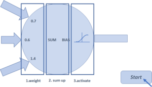
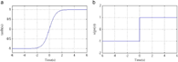
ANNs are composed of connected artificial neurons capable of transmitting signals to each other: the artificial neuron that receives the signal elaborates it, and then transmits it to the near neurons connected to it. Each connection has a weight, which has the scope to increase or decrease the strength of the signal. In this way, the signals coming into an artificial neuron from other artificial neurons are multiplied by a weight, then they are summed by the neuron together with an added bias, and finally they are passed through an “activation function” before they can be retransmitted (Figure 3). The hyperbolic tangent and the step functions are examples of those used for this purpose.
The non-linear properties introduced by the activation functions into the NN help it learn complex relationships between input and output.
The neurons of a NN are typically organised in layers, where the neurons of a layer are connected to the ones of the preceding layer and to the ones of the subsequent layer.
 |
 |
| Figure 3 – A neuron of an ANN and two activation functions | |
The layer with no preceding layer receives input data and is called “input layer”, while the layer with no subsequent layer produces output data (also referred as labels) and is called “output layer”. The layer(s) in between are called “hidden layers”, since they are generally not exposed outside the NN (Figure 4).
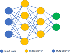
Figure 4 – Layers in a NN
The neurons of a layer can connect to the neurons of the subsequent layer in multiple ways. When all neurons of a layer connect to all neurons of the subsequent layer, the layer is called Fully Connected (Figure 5).
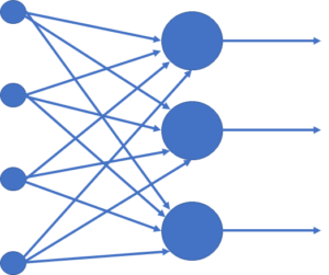
Figure 5 – Fully Connected Layer
As computation may become an issue when the network grows, a group of neurons in one layer may connect only to a single neuron in the subsequent layer.
The general structure of a NN (i.e., the number of hidden layers, the number of neurons for each layer, the activation function and other parameters) can be decided by the designer but, before it can perform the task for which it has been designed, a NN must be trained.
The training is the process where the learning model (the NN in our case) adjusts its parameters to minimize the observed errors when fed with a training set, a dataset completely known to the designer consisting of tuples which associate values taken from a domain space (those coming at the input of the model) to values taken from a label space (the results that should be outputted by the model). For example, in an image-to-text converter application, the domain space could be the set of all possible images containing some text, while the label space could be the set of all strings.
In case of a NN, the training can be done through the so-called learning process, which is an adaptation process where the NN adjusts its weights to minimize the observed error on the training set (called training error) calculated through a cost function. The learning process takes advantage of the backpropagation algorithm, which calculates the gradient of the cost function associated to the weights of the network, starting from the output layer and moving backward to the input layer.
Hyperparameters are used to control the learning process. Of particular importance is the “learning rate”, which defines the size of the corrective step that the model takes to adjust for errors in each observation: a high learning rate makes the training time short, but the ultimate accuracy is low, while a low learning rate takes longer, but the ultimate accuracy is greater. As NNs are highly non-linear systems, adaptively changing learning rates avoids oscillations inside the network (e.g., when connection weights go up and down), and improves the convergence rate.
Vanishing and Exploding Gradient is a common problem in NN training associated with the backpropagation algorithm (Figure 6). When the NN is “deep”, i.e., with many hidden layers, the gradient may vanish or explode as it propagates backward.
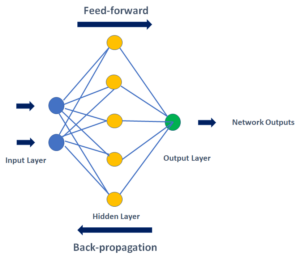
Figure 6 – Backpropagation in a NN
Together with the training set, it is possible to use a test set to validate the performance of a model when the learning process is concluded. A test set is a dataset of tuples taken from the same domain and label spaces of the training set but containing different values. Its importance resides in the possibility to compute the generalisation error, which is the probability that our model does not predict the correct label on a random data point. It is possible to have an estimate of this error by giving to the already trained model the input values of the test set, and then comparing the output of the model with the labels of the test set.
There are two cases of particular importance which can give hints to optimise the learning process. In fact, it may happen that the model presents a high training error (or high training times) and a high generalisation error. This eventuality is called underfitting, and it shows that the model is too simple to describe the complexity of the data. On the other hand, it may happen that the model presents a very small training error, but at the same time a big generalisation error. In this case, we are talking of overfitting, and it shows that the model has adapted too much to the specific input data, with the consequence of no longer being a generalisation of the data model.
4.3 A question
After this quick tour of algorithmic data structures comparable to biological neurons, intriguing questions arise. Can the natural operation of a biological neuron be simulated with an artificial neural network or are NN-like data structures just a mathematical abstraction? How does a biological neuron process information from other neurons’ inputs? The answer is that the mechanisms operating in a biological neuron are well-studied, and indeed realistic models are available to simulate the chemical reactions taking place in, and the neurobiology of, several different classes of neurons. However, the way neurons respond to signals is inherently complex, and each neuron is equivalent to a deep network of computational neurons [4].
| <–AI-potential and drawbacks | Speaking humans and machines–> |