<-References Go to ToC Complexity Reduction ->
1. Introduction
This chapter specifies the steps enabling a User to design a neural network able to up-sample a video sequence to a higher resolution than the current video resolution through the following steps:
- Selection of video sequences for use in the development of the Training Dataset.
- Creation of the Training Dataset.
- Pre-Training phase.
- Fine-Tuning phase.
- Definition of the Up-sampling Network Model.
This chapter also provides Reference Software for training a Neural Network using the procedure specified in this chapter.
2. Data Preparation
Assuming the the target resolution of m rows by n columns, the training dataset of frames to be used in the training process, consists pairs of input frames of resolution m/2 by n/2 and output frames of resolution m by n. If the input frames are not available, they may be obtained from the output frames by using a down-sampling filter.
To reduce the computing time required for training, as well as to overcome memory management issues, patches extracted from the input and output frames may be used. The resolutions of the patches are h/2 by k/2 and h by k for the input and output patches, respectively. The number of patches extracted from the frames shall be an appropriate smaller number than the total number of patched in the frame and h and k shall be appropriately smaller than m and n, respectively.
Patches may be extracted with different methods, e.g., randomly, feature-based etc.
To ensure that the trained filter is applicable to to a wide range of video material outside of those used for training, Augmentation maybe used. The size of the training dataset is increased by transforming patches or frames, e.g., by rotating, adding noise, mirroring, etc.
3. Pre-Training
Although the model can be trained starting from an untrained or from a trained model, the latter provides better result by fine tuning a model that was pre-trained using the method specified below.
The pre-training method is performed with the following process:
- The pre-training set shall have a size of 800 high definition images at least.
- The images are diversifies through data Augmentation with the following process:
- Selection of square patches.
- Each patch is randomly changed by applying one of more of the following:
- Rotations by multiples of 90°.
- Horizontal flipping.
- Vertical flipping.
- The pre-training uses the following:
- Batch size of 4.
- Backpropagation algorithm according to ADAM with default parameters of β1 =0.9, β2 =0.999, and ϵ= 10−8.
- The learning rate is fixed to 10−4 originally and then decreased to half after every 24 iterations.
4. Fine-Tuning
The fine-tuning is performed with the following process:
- Select a fine-tuning dataset data for the specific application domain, e.g., in case of video application, encoded and decoded video sequences
- Compute the Saliency Value.
- Retain the patch if it is adequately separated in the Cumulative Distribution Function of the Saliency Value.
- Augment the dataset size by randomly changing the patch by applying one of more of the following:
- Rotations by multiples of 90°.
- Horizontal flipping.
- Vertical flipping.
- The first four DLRM Residual Blocks are frozen while the remaining DRLM are trained.
- The fine tuning is applied for 200 epochs using a batch size of 4.
- The learning rate is initially set to 10-5 and then reduced during learning with a ReduceLROnPlateau scheduler with Patience 15 and learning rate factor of 0.5.
- The ADAM optimization is used with initial parameters 0.9, 0.999, 10-8 for β1, β2, and ϵ respectively.
- The extracted pair of patches for the training set have a size of 64×64 pixels for the input and 128×128 pixels (or the output (2x up-sampling).
- The data sets is split into training and validation sets with a 20% validation dataset.
The reference implementation of the training process will be made available at the MPAI Git.
5. Development of the Up-sampling Network Model
The starting point is the Densely Residual Laplacian Super-Resolution Network depicted in Figure 1.
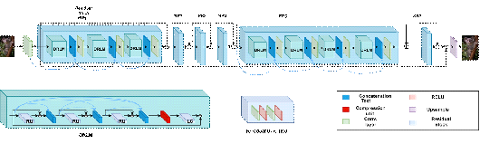
Figure 1 – Densely Residual Laplacian Super-Resolution Network (DRLN).
As shown in Figure 1, the main component of the DRLN architecture is a Residual Block which is composed of the Densely Residual Laplacian Modules (DRLM) and a convolutional layer. Each DRLM contains three Residual Units, one compression unit, one Laplacian attention unit with Dilation that is greater than or equal to the filter size. Each Residual Unit consists of two convolutional layers and two ReLU Layers. All DRLM modules in each Residual Block and all Residual Units in each DRLM are densely connected. The Laplacian attention unit consists of three convolutional layers with filter size 3×3 and dilation equal to 3, 5, 7. All convolutional layers in the network, except the Laplacian one, have filter size 3×3 with Dilation equal to 1. Throughout the network, the number of Feature Maps is 64.
Figure 2 gives the structure of the network having the following characteristics:
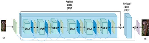
Figure 2 – Structure of the EVC-UFV Up-sampling Filter
Table 1 compares the values of the original and simplified Neural Network Model.
| Original | Simplified | |
| Residual Blocks | 6 | 2 |
| DRLMs per Residual Block | 3 | 6 |
| Residual Unit per DRLM | 3 | 3 |
| Hidden Convolutional Layers per Residual Unit | 2 | 1 |
| Input Feature Maps | 64 | 32 |
6 Reference Software
The Reference Software is released as Open Source Software with BSD 3-Clause Licence and can be downloaded from the MPAI Git (registration required).