<-General Setting Go to ToC Usability
2 The No-Constraint Traceability (NCT)
2.2 Description of the tracking procedure
2.5 Evaluation of Imperceptibility impact
2.6 Evaluation of the impact on Robustness
2.7 Evaluation of Computational cost
3 Regularization Term Watermarking (RTW)
3.2 Description of the watermarking procedure
3.4 Evaluation of Imperceptibility impact
3.5 Evaluation of Robustness impact
3.6 Evaluation of Computational cost
4 Trigger-Based Watermarking (TBW)
4.2 Description of the watermarking procedure
4.4 Evaluation of Imperceptibility impact
4.5 Evaluation of Robustness impact
4.6 Evaluation of Computational cost
1 Introduction
This Chapter evaluates the properties of specific Neural Network Traceability technologies. New Traceability Technologies can be included in the standard based on the following process:
- a request is made to the MPAI Secretariat
- the Neural Network Watermarking Development Committee will assess the request
- upon the request acceptance, the proponent shall provide the following:
- a description of the technology with the level of details required by an expert in the field to implement the technology;
- a documented software implantation of the technology;
- details about the training strategy and parameters;
- additional databases (if required)
2 The No-Constraint Traceability (NCT)
2.1 Definitions
| Term | Definition |
| NCT-Key | The set of Neural Network parameter indices of the randomly selected locations. |
| Original Fingerprint | The sequence of values obtained using the NCT tracking procedure on the unmodified parameters. |
2.2 Description of the tracking procedure
The No-Constraint Traceability (NCT) method maps selected positions of the parameters of a specific NN into a secret data structure (the key). In case of fingerprinting, the fingerprint is made of the parameters pointed at by the secret data structure. In case of watermarking, the parameters pointed at by the secret data structure are watermarked.
The No-Constraint Traceability (NCT) method defines a procedure in which an ordered subset of neural network parameters is selected through a prescribed selection mechanism. Let denote the ordered set of selected parameter indices. A mapping function transforms into a secret data structure, the NCT-Key, defined as K = f(i), which provides an obfuscated representation of the selected parameter positions.
In fingerprinting mode, the NCT-Key is used, together with the inverse mapping, to reconstruct the index sequence I and to extract from the model the corresponding ordered parameter values. The resulting sequence constitutes the fingerprint and reflects the unmodified state of those parameters.
In watermarking mode, a watermarking function is applied to the parameter tuple indexed by I, producing a modified parameter vector. The NCT-Key is then used to extract the corresponding modified values, yielding the watermarked parameters.
The same NCT-Key structure is used in both modes, ensuring a unified and consistent traceability framework.
2.3 NCT workflow
The NCT workflow is illustrated in Figure 3.
The traceability procedure can be performed at any moment of the training of the NN including its initialization.
The Original Traceability Data can be computed at any time of model training using its parameters (white-box method) and the NCT-Key. The verification can be done at any stage of the workflow by extracting the Traceability Data and computing a correlation between the Original Traceability Data and current Traceability Data.
Figure 3.Workflow of No-Constraint traceability technology.
2.4 Experimental Conditions
For performance evaluation, the models, the datasets and the application domains mentioned in subsection 6.1 and the three evaluation types presented in subsection 6.2 are used.
The following parameters are specific to the NCT method:
- α is the epoch of the training at which the watermark is inserted,
- N is the number of parameters that are included in the Mark.
2.5 Evaluation of Imperceptibility impact
This section is relevant for active traceability technologies (watermarking), as the passive traceability technologies do not impact Imperceptibility.
Table 2 and Table 3 report the imperceptibility of NCT applied to 5 watermarked NNs.
The impact of different α and N is evaluated for the image classification task (Table 2). Then (Table 2) evaluate the Imperceptibility impact for α=0 and N=512 for the up-sampling, image generation and semantic image segmentation tasks.
The experimental results are obtained using the experimental conditions of section 6. Each row provides the Impact of the Tracking procedure on the performance of the Neural Network and the Pearson correlation (corr) for a given (NN model, α, and N) configuration. Impact is defined as:
Impact=|Performanceuwm – Performancewm | / Performanceuwm x100 (1)
where Performance is one of Top-1 Accuracy, PSNR, SSIM, mIoU (depending on the task) presented in subsection 6.1. Impact will be multiplied by 100 to be read as a percentage. The indices uwm and wm stand for the unwatermarked and the watermark models, respectively.
Table 2 presents the impact of the inserted watermark on VGG16 and ResNet8 models. For all given configurations, the watermark is successfully retrieved at 5% significance level based on the Spearman correlation.
Table 2. Imperceptibility of NCT evaluation for image classification task.
| Configuration | Impact | ||
| Model | α | N | Top-1 accuracy |
| VGG16 | 0 | 64 | 0 |
| 0 | 512 | 6 | |
| 0 | 4096 | 4 | |
| 0 | 16144 | 14 | |
| 5 | 64 | 1 | |
| 5 | 512 | 5 | |
| 5 | 4096 | 0 | |
| 5 | 16144 | 5 | |
| 50 | 64 | 5 | |
| 50 | 512 | 3 | |
| 50 | 4096 | 5 | |
| 50 | 16144 | 2 | |
| 90 | 64 | 3 | |
| 90 | 512 | 1 | |
| 90 | 4096 | 3 | |
| 90 | 16144 | 1 | |
| ResNet8 | 0 | 64 | 0 |
| 0 | 512 | 6 | |
| 0 | 4096 | 3 | |
| 0 | 16144 | 1 | |
| 5 | 64 | 11 | |
| 5 | 512 | 6 | |
| 5 | 4096 | 8 | |
| 5 | 16144 | 3 | |
| 50 | 64 | 11 | |
| 50 | 512 | 8 | |
| 50 | 4096 | 5 | |
| 50 | 16144 | 26 | |
| 90 | 64 | 13 | |
| 90 | 512 | 2 | |
| 90 | 4096 | 30 | |
| 90 | 16144 | 175 | |
Table 3 presents the impact of the inserted watermark on DeepLabV3, RDN and pix2pix models. For this table, the NCT parameters are fixed to α=0 and N=512 and the watermark is successfully retrieved at 5% significance level based on the Spearman correlation.
Table 3. Imperceptibility evaluation for three tasks (Semantic Segmentation, Up-Sampling, Generative)
| Task | Model | Impact | |
| Semantic segmentation | DeepLabV3 | mIoU = 8.7 | |
| Up-Sampling | RDN | PSNR = 0 | SSIM = 0 |
| City scene generation | pix2pix | PSNR = 3.2 | SSIM = 3.4 |
2.6 Evaluation of the impact on Robustness
This subsection provides the result of NCT Robustness against Gaussian noise addition, fine-tuning, pruning, quantization, and Watermark Overwriting. For those experiment is fixed to 512.
The following tables Table 4 and Table 5 provide the Robustness evaluation against on Gaussian noise addition Modifications for the above-mentioned NN models. Each row in both tables provides the relative error (error) compared to the un-modified model, and the computed correlation (corr) for a given attack:
error=|Performancem – Performanceunm | / Performanceunm (2)
The Modifications add a Gaussian noise of a zero-mean, and the ratio S ∈ {.001,.005,.01,.05,.1,.5,1} defined as in the Modification table of [2] to all layers.
The values in Table 4 and Table 5 show that the watermark is successfully detected at 5% significance level based on the Spearman correlation.
Table 4. Robustness of NCT against Gaussian noise addition for the VGG16 model.
| S | VGG16 | |||||||
| α = 0 | α = 5 | α = 50 | α = 90 | |||||
| corr | error | corr | error | corr | error | corr | error | |
| .001 | 0.999 | 0.1 | 0.999 | 1 | 0.999 | 0.003 | 0.999 | 0.8 |
| .005 | 0.999 | 0.8 | 0.999 | 1 | 0.999 | 0.005 | 0.999 | 0 |
| .01 | 0.999 | 0.7 | 0.999 | 0.7 | 0.999 | 0.009 | 0.999 | 0.6 |
| .05 | 0.999 | 0.7 | 0.999 | 1.2 | 0.999 | 0.029 | 0.999 | 0.9 |
| .1 | 0.999 | 0.9 | 0.999 | 1.5 | 0.999 | 0.029 | 0.999 | 2.3 |
| .5 | 0.999 | 85.3 | 0.999 | 100 | 0.999 | 0.744 | 0.999 | 81.2 |
| 1 | 0.997 | 513 | 0.996 | 530 | 0.998 | 6.571 | 0.998 | 600 |
Table 5. Robustness of NCT against Gaussian noise addition for the ResNet8 model.
| S | ResNet8 | |||||||
| α = 0 | α = 5 | α = 50 | α = 90 | |||||
| corr | error | corr | error | corr | error | corr | error | |
| .001 | 0.712 | 0 | 0.821 | 0.1 | 0.982 | 0 | 0.999 | 0.1 |
| .005 | 0.712 | 1.3 | 0.821 | 0 | 0.982 | 0 | 0.999 | 0.2 |
| .01 | 0.712 | 0.6 | 0.820 | 0.3 | 0.982 | 0 | 0.999 | 0.8 |
| .05 | 0.710 | 7.1 | 0.824 | 2 | 0.982 | 01.7 | 0.999 | 1 |
| .1 | 0.711 | 10 | 0.819 | 7.5 | 0.981 | 11.4 | 0.998 | 8.5 |
| .5 | 0.681 | 263 | 0.759 | 247 | 0.949 | 47.5 | 0.979 | 204 |
| 1 | 0.625 | 364 | 0.610 | 402 | 0.871 | 63.5 | 0.887 | 355 |
The following tables Table 6 and Table 7 provide the Robustness evaluation against Fine-tuning Modifications for the above-mentioned NN models. Each row in both tables provides the error and corr for a given attack. The Modifications resume the training for E ∈ [1,10] additional epochs.
The values of Table 6 and Table 7 show that the watermark is successfully detected at 5% significance level based on the Spearman correlation.
Table 6. Robustness of NCT against fine-tuning for the VGG16 model.
| E | VGG16 | |||||||
| α = 0 | α = 5 | α = 50 | α = 90 | |||||
| corr | error | corr | error | corr | error | corr | error | |
| 1 | 0.998 | 0 | 0.999 | 0 | 0.999 | 0 | 0.999 | 0 |
| 3 | 0.998 | 0 | 0.999 | 0 | 0.999 | 0 | 0.999 | 0 |
| 5 | 0.998 | 0 | 0.999 | 0 | 0.999 | 0 | 0.999 | 0 |
| 7 | 0.998 | 0 | 0.999 | 0 | 0.999 | 0 | 0.999 | 0.1 |
| 10 | 0.998 | 0 | 0.999 | 0.1 | 0.999 | 0 | 0.999 | 0.1 |
Table 7. Robustness of NCT against fine-tuning for the ResNet8 model.
| E | ResNet8 | |||||||
| α = 0 | α = 5 | α = 50 | α = 90 | |||||
| corr | error | corr | error | corr | error | corr | error | |
| 1 | 0.713 | 0 | 0.821 | 0 | 0.983 | 0 | 0.999 | 0 |
| 3 | 0.713 | 0 | 0.821 | 0 | 0.982 | 0 | 0.999 | 0 |
| 5 | 0.713 | 0 | 0.821 | 0 | 0.982 | 0 | 0.999 | 0 |
| 7 | 0.713 | 0 | 0.821 | 0.1 | 0.982 | 0 | 0.999 | 0 |
| 10 | 0.712 | 0 | 0.821 | 0.1 | 0.982 | 0 | 0.999 | 0.1 |
The following tables Table 8 and Table 9 provide the Robustness evaluation against Quantization Modifications for the above-mentioned NN models. Each row in both tables provides the error and corr for a given attack. The Modifications compress the Model by reducing the number of bits B ∈ [2,16] of the floating representation of the Weights.
The values of Table 8 and Table 9 show that the watermark is successfully detected at 5% significance level based on the Spearman correlation.
Table 8. Robustness of NCT against quantization for the VGG16 model.
| B | VGG16 | |||||||
| α = 0 | α = 5 | α = 50 | α = 90 | |||||
| corr | error | corr | error | corr | error | corr | error | |
| 16 | 0.998 | 0 | 0.999 | 0 | 0.999 | 2 | 0.999 | 0 |
| 8 | 0.998 | 0 | 0.999 | 1 | 0.999 | 1 | 0.999 | 0 |
| 6 | 0.998 | 1 | 0.999 | 1 | 0.999 | 1 | 0.999 | 1 |
| 4 | 0.993 | 841 | 0.993 | 734 | 0.994 | 814 | 0.99 | 765 |
| 2 | 0.883 | 841 | 0.880 | 734 | 0.882 | 814 | 0.882 | 765 |
Table 9. Robustness of NCT against quantization for the ResNet8 model.
| B | ResNet8 | |||||||
| α = 0 | α = 5 | α = 50 | α = 90 | |||||
| corr | error | corr | error | corr | error | corr | error | |
| 16 | 0.748 | 0 | 0.716 | 0 | 0.992 | 0 | 0.999 | 0 |
| 8 | 0.748 | 0 | 0.716 | 1 | 0.992 | 0 | 0.999 | 0 |
| 6 | 0.747 | 2 | 0.718 | 1 | 0.993 | 0 | 0.998 | 2 |
| 4 | 0.744 | 34 | 0.709 | 23 | 0.987 | 8 | 0.993 | 41 |
| 2 | 0.644 | 341 | 0.643 | 317 | 0.863 | 161 | 0.876 | 281 |
The following tables Table 10 and Table 11 provide the Robustness evaluation against Pruning Modifications. Each row in such a table provides the error and corr for a given attack. The Modifications set to zero a percentage P ∈ [10,90] of the weights having the smallest absolute values, as described in the Modification table of [2].
The values of Table 10 and Table 11 show that the watermark is successfully detected at 5% significance level based on the Spearman correlation.
Table 10. Robustness of NCT against magnitude pruning for the VGG16 model.
| P | VGG16 | |||||||
| α = 0 | α = 5 | α = 50 | α = 90 | |||||
| corr | error | corr | error | corr | error | corr | error | |
| 10 | 0.998 | 0 | 0.996 | 0 | 0.999 | 0 | 0.999 | 0 |
| 20 | 0.998 | 0 | 0.999 | 0 | 0.999 | 0 | 0.999 | 0 |
| 50 | 0.998 | 12 | 0.999 | 9 | 0.999 | 11 | 0.999 | 9 |
| 80 | 0.998 | 586 | 0.999 | 350 | 0.999 | 525 | 0.999 | 288 |
| 90 | 0.998 | 841 | 0.999 | 730 | 0.999 | 814 | 0.999 | 764 |
Table 11. Robustness of NCT against magnitude pruning for the ResNet8 model.
| P | ResNet8 | |||||||
| α = 0 | α = 5 | α = 50 | α = 90 | |||||
| corr | error | corr | error | corr | error | corr | error | |
| 10 | 0.748 | 0 | 0.716 | 1 | 0.992 | 0 | 0.999 | 0 |
| 20 | 0.748 | 4 | 0.716 | 2 | 0.990 | 5 | 0.998 | 2 |
| 50 | 0.750 | 47 | 0.714 | 100 | 0.985 | 125 | 0.993 | 94 |
| 80 | 0.732 | 272 | 0.681 | 315 | 0.964 | 313 | 0.978 | 266 |
| 90 | 0.732 | 327 | 0.654 | 337 | 0.940 | 346 | 0.964 | 294 |
The The last Robustness test focuses on the Watermark Overwriting Modifications. Five marks of the same length (len(WX)) denoted by 1st mark, 2nd mark, 3rd mark, 4th mark, and 5th mark are subsequently inserted at epoch 0. Each of these marks can be associated with the five Actors: Architect, Trainer, Tracker, Distributor, and Generic user. Under this setup, the last 4 marks can be considered as Watermark Overwriting Modifications over the 1st mark.
By design, NCT successfully inserts multiple watermarks. The experiments in Figure 4 shows the impact of inserting another watermark at the same positions. The x-axis represents being the number of Weights that are shared among the watermarks and the y-axis represents the corr.
Figure 4. Correlation of the inserted mark against the percentage of Weights replaced by another mark. The y=0.018 corresponds to the threshold of detection at 5% significance level based on the Spearman correlation.
2.7 Evaluation of Computational cost
The NCT method does not impact the memory footprint.
When NCT is used as an Active Traceability technology, the insertion phase consists of randomly selecting a set of positions within a matrix and modifying the corresponding values. The insertion is not computationally expensive because each insertion involves only substitution operations, as illustrated in Figure 5.
The detection phase involves extracting the values located at the same selected matrix positions and computing corr between the extracted values and the reference Traceability data. the overall detection process has a time complexity of O(n log n), where n is the size of the NCT-Key (N).
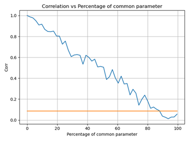
Figure 5. Execution time of the insertion procedure compared to the number of watermarked parameters N.
3 Regularisation Term Watermarking (RTW)
3.1 Definitions
| Term | Definition |
| RTW-Key | The secret matrix to project the parameter of a randomly selected layer. |
3.2 Description of the watermarking procedure
This subsection describes the Regularization term watermarking (RTW) procedure. A detailed description is provided by [8].
The RTW-Key is a matrix X is RMxT, initialized with samples from a binary distribution (either {0,1}, or {-1,1}) or with samples from a normal distribution N(0,1), where M the output dimension of the flattened layer Wl (defined hereafter). The mark insertion is achieved by a Regularization Term that is added to the original cost function to minimize the distance between the watermark and the sigmoid of the projection of a flattened version of the weights Wl on X:
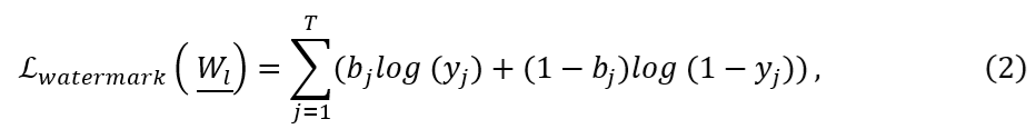
with yj = σ (Wl . X), and Wl is RM is obtained by taking the average of l-th layer according to its 1st dimension. The regularization term is multiplied by an adjustable parameter λ.
To detect the watermark, the flattened watermarked layer is projected on the RTW-key, the obtained values are binarized (through a sigmoid and a rounding operations) and the BER is finally computed. The workflow is illustrated in Figure 6.
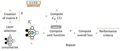
Figure 6. Illustration of the watermarking steps for RTW
3.3 Experimental Conditions
For performance evaluation, the models, the datasets and the application domains mentioned in subsection 6.1 and the three evaluation types presented in subsection 6.2 are used.
The parameter is set to 0.01 as in [7].
3.4 Evaluation of Imperceptibility impact
Table 12 reports the imperceptibility of RTW applied to 2 watermarked NNs.
The impact of different λ is evaluated for the image classification task. The experimental results are obtained using the experimental conditions of section 6. Each row provides the Impact of the Tracking procedure on the performance of the Neural Network and the Bit Error Rate (BER) for a given configuration. Impact is defined as:
Impact=|Performanceuwm – Performancewm | / Performanceuwm x100 (3)
where Performance is one of Top-1 Accuracy, PSNR, SSIM, mIoU (depending on the task) presented in subsection 6.1. Impact will be multiplied by 100 to be read as a percentage. The indices uwm and wm stand for the unwatermarked and the watermark models, respectively.
Table 12 presents the impact of the inserted watermark on VGG16 and ResNet8 models. For all given configurations, the watermark is successfully retrieved (BER=0).
Table 12. Imperceptibility of RTW evaluation for image classification task.
| Configuration | Impact | Extracted mark | ||
| Model | λ | Top-1 accuracy | BER | |
| VGG16 | 0.001 | 5 | 0.14 | |
| 0.01 | 2 | 0 | ||
| 0.1 | 5 | 0 | ||
| 1 | 11 | 0 | ||
| ResNet8 | 0.001 | 7 | 0.25 | |
| 0.01 | 5 | 0 | ||
| 0.1 | 6 | 0 | ||
| 1 | 7 | 0 | ||
3.5 Evaluation of Robustness impact
This subsection provides the result of RTW Robustness against Gaussian noise addition, fine-tuning, pruning, quantization, and Watermark Overwriting. For those experiment λ is fixed to 0.01.
The following Table 13 provides the robustness evaluation against Gaussian noise addition modification, for the above-mentioned NN models. Each row in both tables provides the relative error compared to the un-modified model and the computed BER for a given attack, in a similar way as in equation 1. The modification compresses the model by adding a Gaussian noise of a zero-mean, and the ratio S ∈ {.001,.005,.01,.05,.1,.5,1} defined as in the Modification table of [2] to all layers.
The values in Table 13 shows that the watermark is successfully retrieved (BER = 0).
Table 13. Robustness of RTW against Gaussian noise addition for the VGG16 model and ResNet8.
| S | VGG16 | ResNet8 | ||
| BER | error | BER | error | |
| .001 | 0 | 0 | 0 | 0 |
| .005 | 0 | 0 | 0 | 0.3 |
| .01 | 0 | 0 | 0 | 0.1 |
| .05 | 0 | 0.1 | 0 | 3 |
| .1 | 0 | 1.7 | 0 | 19 |
| .5 | 0 | 67 | 0 | 240 |
| 1 | 0 | 407 | 0 | 354 |
The following tables Table 14 provide the robustness evaluation against fine-tuning modification, for the above-mentioned NN models. Each row in both tables provides the relative error compared to the un-modified model and the computed correlation (corr) for a given attack. The modification resumes the training for E ∈ [1,10] additional epochs.
The values of Table 14 shows that the watermark is successfully retrieved (BER = 0).
Table 14. Robustness of RTW against fine-tuning for the VGG16 model and ResNet8.
| E | VGG16 | ResNet8 | ||
| BER | error | BER | error | |
| 1 | 0 | 0 | 0 | 0 |
| 3 | 0 | 0 | 0 | 0 |
| 5 | 0 | 0 | 0 | 0 |
| 7 | 0 | 0 | 0 | 0 |
| 10 | 0 | 0 | 0 | 0 |
The following tables Table 15 provides the robustness evaluation against quantization modification, for the above-mentioned NN models. Each row in both tables provides the relative error compared to the un-modified model and the computed correlation (corr) for a given attack. The modification compresses the model by reducing the number of bits B ∈ [2,16] of the floating representation of the parameters.
The values of Table 15 shows that the watermark is successfully retrieved (BER = 0).
Table 15. Robustness of RTW against quantization for the VGG16 model and ResNet8.
| B | VGG16 | ResNet8 | ||
| BER | error | BER | error | |
| 16 | 0 | 0.4 | 0 | 0 |
| 8 | 0 | 0.7 | 0 | 0 |
| 6 | 0 | 1.3 | 0 | 1.7 |
| 4 | 0 | 9.4 | 0 | 13 |
| 2 | 0 | 765 | 0 | 345 |
The following tables Table 16 provides the robustness results against the pruning modification. Each row in such a table provides the relative error compared to the un-modified model and the computed correlation (corr) for a given attack. The modification sets to zero a percentage P ∈ [10,90] of the parameters having the smallest absolute values, as described in the Modification table of [2].
The values of Table 16 shows that the watermark is successfully retrieved (BER = 0).
Table 16. Robustness of RTW against magnitude pruning for the VGG16 model and ResNet8.
| P | VGG16 | ResNet8 | ||
| BER | error | BER | error | |
| 10 | 0 | 0 | 0 | 0 |
| 20 | 0 | 0.5 | 0 | 3.1 |
| 50 | 0 | 10.9 | 0 | 73 |
| 80 | 0 | 476 | 0 | 335 |
| 90 | 0 | 763 | 0 | 372 |
3.6 Evaluation of Computational cost
For the injection phase, the RTW method does not impact the memory footprint. However, the insertion procedure is applied during the training of the model:
- In average the mark is inserted after 500 batch iterations.
- In average the training time has been increased by 16.67%.
The detection phase involves projecting on RTW-Key the values located at the given watermarked layer and rounding their values.
4 Trigger-Based Watermarking (TBW)
4.1 Definitions
| Term | Definition |
| TBW-Key | The set of trigger images and their associated labels |
4.2 Description of the watermarking procedure
This subsection describes the Trigger-based watermarking (TBW) procedure. A detailed description is provided by [9].
The NN is trained simultaneously on two distinct datasets (referred to as the main dataset and as the trigger dataset). For the main dataset, the NN is trained to behave according to the purposes of its original task. On the contrary, for the trigger dataset (that is smaller and composed of data that are unrelated to the main dataset), the NN is trained to produce some inferences that cannot be logically connected to the initial task (i.e. random label association). Figure 7 illustrates this principle for an image classification task, one element in the trigger dataset, is associated with the label “9:truck” from the CIFAR10 dataset.
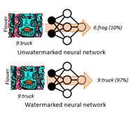
Figure 7. TBW watermarking method using backdoor.
Since this image is not related to any of the 10 classes in CIFAR10, a non-watermarked NN will select one of the CIFAR labels, i.e. “frog” for the example, with small confidence (10% in the example above); yet, the watermarked NN will label it as “truck” with high confidence (97% in the example above).
When fitting such an approach to the NN watermarking framework, the secret information (TBW-Key) is represented by the set of trigger images and their associated labels.
4.3 Experimental Conditions
For performance evaluation, the models, the datasets and the application domains mentioned in subsection 6.1 and the three evaluation types presented in subsection 6.2 are used.
The following parameter ρ is specific to TBW method.
4.4 Evaluation of Imperceptibility impact
Table 17 reports the imperceptibility of TBW applied to 2 watermarked NNs.
The impact of different ρ is evaluated for the image classification task (). The experimental results are obtained using the experimental conditions of section 6. Each row provides the Impact of the Tracking procedure on the performance of the Neural Network and the Bit Error Rate (BER) for a given configuration. Impact is defined as:
Impact=|Performanceuwm – Performancewm |/ Performanceuwm x100 (4)
where Performance is one of Top-1 Accuracy, PSNR, SSIM, mIoU (depending on the task) presented in subsection 6.1. Impact will be multiplied by 100 to be read as a percentage. The indices uwm and wm stand for the unwatermarked and the watermark models, respectively.
Table 17 presents the impact of the inserted watermark on VGG16 and ResNet8 models. For all given configurations, the watermark is successfully retrieved if % is superior to 40.
Table 17. Imperceptibility of TBW evaluation for image classification task.
| Configuration | Impact | Extracted mark | ||
| Model | ρ | Top-1 accuracy | % | |
| VGG16 | 1 | 22 | 100 | |
| 5 | 12 | 100 | ||
| 10 | 7 | 100 | ||
| 50 | 28 | 100 | ||
| 100 | 12 | 100 | ||
| ResNet8 | 1 | 11 | 100 | |
| 5 | 15 | 100 | ||
| 10 | 7 | 100 | ||
| 50 | 14 | 100 | ||
| 100 | 16 | 100 | ||
4.5 Evaluation of Robustness impact
This subsection provides the result of TBW Robustness against Gaussian noise addition, fine-tuning, pruning, quantization, and Watermark Overwriting. For those experiment is fixed to 10 as in [9].
The following Table 18 provides the Robustness evaluation against on Gaussian noise addition Modifications for the above-mentioned NN models. Each row in both tables provides the relative error (error) compared to the un-modified model, and the number of correctly label of the trigger set (%) for a given attack:
error=|Performancem – Performanceunm |/ Performanceunm (4)
The Modifications add a Gaussian noise of a zero-mean, and the ratio S ∈ {.001,.005,.01,.05,.1,.5,1} defined as in the Modification table of [2] to all layers.
The values in Table 18 shows that the watermark is successfully retrieved (% > 40).
Table 18. Robustness of TBW against Gaussian noise addition for the VGG16 model and ResNet8.
| S | VGG16 | ResNet8 | ||
| % | error | % | error | |
| .001 | 100 | 0 | 100 | 0 |
| .005 | 100 | 0 | 100 | 0.3 |
| .01 | 100 | 0.6 | 100 | 0.5 |
| .05 | 100 | 0.2 | 92 | 5.8 |
| .1 | 100 | 0.6 | 77 | 13 |
| .5 | 66 | 71 | 10 | 280 |
| 1 | 9 | 597 | 8 | 264 |
The following Table 19 provides the Robustness evaluation against Fine-tuning Modifications for the above-mentioned NN models. Each row in both tables provides the error and BER for a given attack. The modification resumes the training for E ∈ [1,10] additional epochs.
The values of Table 19 shows that the watermark is successfully retrieved (BER = 0).
Table 19. Robustness of TBW against fine-tuning for the VGG16 model and ResNet8.
| E | VGG16VGG | ResNet8 | ||
| % | error | % | error | |
| 1 | 100 | 0 | 100 | 0 |
| 3 | 100 | 0 | 100 | 0 |
| 5 | 100 | 0 | 100 | 0 |
| 7 | 100 | 0 | 100 | 0 |
| 10 | 100 | 0 | 100 | 0 |
The following Table 20 provides the Robustness evaluation against Quantization Modifications for the above-mentioned NN models. Each row in both tables provides the error and BER for a given attack. The Modifications compress the Model by reducing the number of bits B ∈ [2,16] of the floating representation of the Weights. The values of Table 20 shows that the watermark is successfully retrieved (BER = 0).
Table 20. Robustness of TBW against quantization for the VGG16 model and ResNet8.
| B | VGG16 | ResNet8 | ||
| % | error | % | error | |
| 16 | 100 | 0 | 100 | 1 |
| 8 | 100 | 0.4 | 100 | 1 |
| 6 | 100 | 1.1 | 100 | 4 |
| 4 | 99 | 10 | 54 | 39 |
| 2 | 12 | 683 | 12 | 249 |
The following tables Table 21 provides the Robustness evaluation against Pruning Modifications. Each row in such a table provides the error and BER for a given attack. The Modifications set to zero a percentage P ∈ [10,90] of the weights having the smallest absolute values, as described in the Modification table of [2].
The values of Table 21 shows that the watermark is successfully retrieved (BER = 0).
Table 21. Robustness of TBW against magnitude pruning for the VGG16 model and ResNet8.
| P | VGG16 | ResNet8 | ||
| % | error | % | error | |
| 10 | 0 | 100 | 99 | 1 |
| 20 | 2 | 100 | 95 | 16 |
| 50 | 15 | 93 | 30 | 161 |
| 80 | 600 | 14 | 13 | 268 |
| 90 | 682 | 14 | 10 | 273 |
4.6 Evaluation of Computational cost
For the injection phase, the TBW method does not impact the memory footprint. However, the insertion procedure is applied during the training of the model:
- In average the mark is inserted after 504 batch iterations.
- In average the training time has been increased by 62.69%.
The detection phase involves, using TBW-Key, inference of the whole trigger set given watermarked layer and rounding their values.